The Central Limit Theorem for Sums

Suppose X is a random variable with a distribution that may be known or unknown (it can be any distribution) and suppose:

If you draw random samples of size n, then as n increases, the random variable ΣX consisting of sums tends to be normally distributed and ΣΧ ~ N((n)(μ_Χ), (

\sqrt{n}

The central limit theorem for sums says that if you keep drawing larger and larger samples and taking their sums, the sums form their own normal distribution (the sampling distribution), which approaches a normal distribution as the sample size increases. The normal distribution has a mean equal to the original mean multiplied by the sample size and a standard deviation equal to the original standard deviation multiplied by the square root of the sample size.

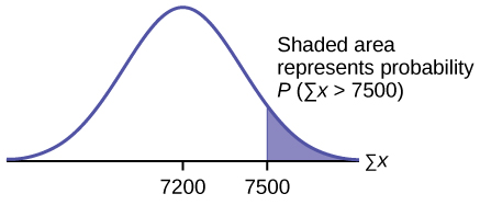
An unknown distribution has a mean of 90 and a standard deviation of 15. A sample of size 80 is drawn randomly from the population.* * *

Find the probability that the sum of the 80 values (or the total of the 80 values) is more than 7,500.
Find the sum that is 1.5 standard deviations above the mean of the sums.

Let X = one value from the original unknown population. The probability question asks you to find a probability for the sum (or total of) 80 values.

ΣX = the sum or total of 80 values. Since μ_X = 90, σ_X = 15, and n = 80, $Σ X$

~ N((80)(90), * * *

( $\sqrt{80}$

)(15))

mean of the sums = (n)(μ_X) = (80)(90) = 7,200
standard deviation of the sums = $(\sqrt{n})(σ_{X}) = (\sqrt{80})$
(15)
sum of 80 values = Σx = 7,500

a. Find P(Σx > 7,500)

P(Σx > 7,500) = 0.0127

This is a normal distribution curve. The peak of the curve coincides with the point 7200 on the horizontal axis. The point 7500 is also labeled. A vertical line extends from point 7500 to the curve. The area to the right of 7500 below the curve is shaded. {:}

normalcdf(lower value, upper value, mean of sums, stdev of sums)

The parameter list is abbreviated(lower, upper, (n)(μ_X, $(\sqrt{n})$

(σ_X))

normalcdf (7500,1E99,(80)(90), $(\sqrt{80})$

(15)) = 0.0127

Reminder

1E99 = 10⁹⁹.

Press the EE key for E.

b. Find Σx where z = 1.5.

Σx = (n)(μ_X) + (z) $(\sqrt{n})$

(σ_Χ) = (80)(90) + (1.5)( $\sqrt{80}$

)(15) = 7,401.2

In a recent study reported Oct. 29, 2012 on the Flurry Blog, the mean age of tablet users is 34 years. Suppose the standard deviation is 15 years. The sample of size is 50.

What are the mean and standard deviation for the sum of the ages of tablet users? What is the distribution?
Find the probability that the sum of the ages is between 1,500 and 1,800 years.
Find the 80^th percentile for the sum of the 50 ages.

μ_Σx = nμ_x = 50(34) = 1,700 and σ_Σx = $\sqrt{n}$
σ_x =
$(\sqrt{50})$
(15) = 106.07

The distribution is normal for sums by the central limit theorem.
P(1500 < Σx < 1800) = normalcdf (1,500, 1,800, (50)(34), $(\sqrt{50})$
(15)) = 0.7974
Let k = the 80^th percentile.

k = invNorm(0.80,(50)(34),
$(\sqrt{50})$
(15)) = 1,789.3

The mean number of minutes for app engagement by a tablet user is 8.2 minutes. Suppose the standard deviation is one minute. Take a sample of size 70.

What are the mean and standard deviation for the sums?
Find the 95^th percentile for the sum of the sample. Interpret this value in a complete sentence.
Find the probability that the sum of the sample is at least ten hours.

μ_Σx = nμ_x = 70(8.2) = 574 minutes and σ_Σx = $(\sqrt{n}) (σ_{x})$
=
$(\sqrt{70})$
(1) = 8.37 minutes
Let k = the 95^th percentile.

k = invNorm (0.95,(70)(8.2),
$(\sqrt{70})$
(1)) = 587.76 minutes

Ninety five percent of the sums of app engagement times are at most 587.76 minutes.
ten hours = 600 minutes

P(Σx ≥ 600) = normalcdf(600,E99,(70)(8.2),
$(\sqrt{70})$
(1)) = 0.0009

References

Farago, Peter. “The Truth About Cats and Dogs: Smartphone vs Tablet Usage Differences.” The Flurry Blog, 2013. Posted October 29, 2012. Available online at http://blog.flurry.com (accessed May 17, 2013).

Chapter Review

The central limit theorem tells us that for a population with any distribution, the distribution of the sums for the sample means approaches a normal distribution as the sample size increases. In other words, if the sample size is large enough, the distribution of the sums can be approximated by a normal distribution even if the original population is not normally distributed. Additionally, if the original population has a mean of μ_X and a standard deviation of σ_x, the mean of the sums is nμ_x and the standard deviation is

(\sqrt{n})

Formula Review

The Central Limit Theorem for Sums z-score and standard deviation for sums:

z for the sample mean = \frac{Σ x - (n) (μ_{X})}{(\sqrt{n}) (σ_{X})}

Use the following information to answer the next four exercises: An unknown distribution has a mean of 80 and a standard deviation of 12. A sample size of 95 is drawn randomly from the population.

Find the probability that the sum of the 95 values is greater than 7,650.

0.3345

Find the probability that the sum of the 95 values is less than 7,400.

Find the sum that is two standard deviations above the mean of the sums.

7,833.92

Find the sum that is 1.5 standard deviations below the mean of the sums.

Use the following information to answer the next five exercises: The distribution of results from a cholesterol test has a mean of 180 and a standard deviation of 20. A sample size of 40 is drawn randomly.

Find the probability that the sum of the 40 values is greater than 7,500.

0.0089

Find the probability that the sum of the 40 values is less than 7,000.

Find the sum that is one standard deviation above the mean of the sums.

7,326.49

Find the sum that is 1.5 standard deviations below the mean of the sums.

Find the percentage of sums between 1.5 standard deviations below the mean of the sums and one standard deviation above the mean of the sums.

77.45%

Use the following information to answer the next six exercises: A researcher measures the amount of sugar in several cans of the same soda. The mean is 39.01 with a standard deviation of 0.5. The researcher randomly selects a sample of 100.

Find the probability that the sum of the 100 values is greater than 3,910.

Find the probability that the sum of the 100 values is less than 3,900.

0.4207

Find the probability that the sum of the 100 values falls between the numbers you found in [link] and [link].

Find the sum with a z–score of –2.5.

3,888.5

Find the sum with a z–score of 0.5.

Find the probability that the sums will fall between the z-scores –2 and 1.

0.8186

Use the following information to answer the next four exercises: An unknown distribution has a mean 12 and a standard deviation of one. A sample size of 25 is taken. Let X = the object of interest.

What is the mean of ΣX?

What is the standard deviation of ΣX?

What is P(Σx = 290)?

What is P(Σx > 290)?

0.9772

True or False: only the sums of normal distributions are also normal distributions.

In order for the sums of a distribution to approach a normal distribution, what must be true?

The sample size, n, gets larger.

What three things must you know about a distribution to find the probability of sums?

An unknown distribution has a mean of 25 and a standard deviation of six. Let X = one object from this distribution. What is the sample size if the standard deviation of ΣX is 42?

An unknown distribution has a mean of 19 and a standard deviation of 20. Let X = the object of interest. What is the sample size if the mean of ΣX is 15,200?

Use the following information to answer the next three exercises.* A market researcher analyzes how many electronics devices customers buy in a single purchase. The distribution has a mean of three with a standard deviation of 0.7. She samples 400 customers.

What is the z-score for Σx = 840?

26.00

What is the z-score for Σx = 1,186?

What is P(Σx < 1,186)?

0.1587

Use the following information to answer the next three exercises:* An unkwon distribution has a mean of 100, a standard deviation of 100, and a sample size of 100. Let X = one object of interest.

What is the mean of ΣX?

What is the standard deviation of ΣX?

1,000

What is P(Σx > 9,000)?

Homework

Salaries for teachers in a particular elementary school district are normally distributed with a mean of $44,000 and a standard deviation of $6,500. We randomly survey ten teachers from that district.

In words, X = ______________
X ~ _____(_____,_____)
In words, ΣX = _____________
ΣX ~ _____(_____,_____)
Find the probability that the teachers earn a total of over $400,000.
Find the 90^th percentile for an individual teacher’s salary.
Find the 90^th percentile for the sum of ten teachers’ salary.
If we surveyed 70 teachers instead of ten, graphically, how would that change the distribution in part d?
If each of the 70 teachers received a $3,000 raise, graphically, how would that change the distribution in part b?

X = the salary of one elementary school teacher in the district
X ~ N(44,000, 6,500)
ΣX ~ sum of the salaries of ten elementary school teachers in the sample
ΣX ~ N(44000, 20554.80)
0.9742
$52,330.09
466,342.04
Sampling 70 teachers instead of ten would cause the distribution to be more spread out. It would be a more symmetrical normal curve.
If every teacher received a $3,000 raise, the distribution of X would shift to the right by $3,000. In other words, it would have a mean of $47,000.