Second-Order Linear Equations
- Recognize homogeneous and nonhomogeneous linear differential equations.
- Determine the characteristic equation of a homogeneous linear equation.
- Use the roots of the characteristic equation to find the solution to a homogeneous linear equation.
- Solve initial-value and boundary-value problems involving linear differential equations.
When working with differential equations, usually the goal is to find a solution. In other words, we want to find a function (or functions) that satisfies the differential equation. The technique we use to find these solutions varies, depending on the form of the differential equation with which we are working. Second-order differential equations have several important characteristics that can help us determine which solution method to use. In this section, we examine some of these characteristics and the associated terminology.
Homogeneous Linear Equations
Consider the second-order differential equation
Notice that y and its derivatives appear in a relatively simple form. They are multiplied by functions of x, but are not raised to any powers themselves, nor are they multiplied together. As discussed in Introduction to Differential Equations, first-order equations with similar characteristics are said to be linear. The same is true of second-order equations. Also note that all the terms in this differential equation involve either y or one of its derivatives. There are no terms involving only functions of x. Equations like this, in which every term contains y or one of its derivatives, are called homogeneous.
Not all differential equations are homogeneous. Consider the differential equation
The
term on the right side of the equal sign does not contain y or any of its derivatives. Therefore, this differential equation is nonhomogeneous.
Definition
A second-order differential equation is linear if it can be written in the form
where
and
are real-valued functions and
is not identically zero. If
—in other words, if
for every value of x—the equation is said to be a homogeneous linear equation. If
for some value of
the equation is said to be a nonhomogeneous linear equation.
In linear differential equations,
and its derivatives can be raised only to the first power and they may not be multiplied by one another. Terms involving
or
make the equation nonlinear. Functions of
and its derivatives, such as
or
are similarly prohibited in linear differential equations.
Note that equations may not always be given in standard form (the form shown in the definition). It can be helpful to rewrite them in that form to decide whether they are linear, or whether a linear equation is homogeneous.
Classifying Second-Order Equations
Classify each of the following equations as linear or nonlinear. If the equation is linear, determine further whether it is homogeneous or nonhomogeneous.
-
-
-
-
-
-
-
-
- This equation is nonlinear because of the
term.
- This equation is linear. There is no term involving a power or function of
and the coefficients are all functions of
The equation is already written in standard form, and
is identically zero, so the equation is homogeneous.
- This equation is nonlinear. Note that, in this case, x is the dependent variable and t is the independent variable. The second term involves the product of
and
so the equation is nonlinear.
- This equation is linear. Since
the equation is nonhomogeneous.
- This equation is nonlinear, because of the
term.
- This equation is linear. Rewriting it in standard form gives
With the equation in standard form, we can see that
so the equation is nonhomogeneous.
- This equation looks like it’s linear, but we should rewrite it in standard form to be sure. We get
This equation is, indeed, linear. With
it is nonhomogeneous.
- This equation is nonlinear because of the
term.
Classify each of the following equations as linear or nonlinear. If the equation is linear, determine further whether it is homogeneous or nonhomogeneous.
-
-
- Nonlinear
- Linear, nonhomogeneous
Hint
Write the equation in standard form if necessary. Check for powers or functions of
and its derivatives.
Later in this section, we will see some techniques for solving specific types of differential equations. Before we get to that, however, let’s get a feel for how solutions to linear differential equations behave. In many cases, solving differential equations depends on making educated guesses about what the solution might look like. Knowing how various types of solutions behave will be helpful.
Verifying a Solution
Consider the linear, homogeneous differential equation
Looking at this equation, notice that the coefficient functions are polynomials, with higher powers of
associated with higher-order derivatives of
Show that
is a solution to this differential equation.
Let
Then
and
Substituting into the differential equation, we see that
Show that
is a solution to the differential equation
Hint
Calculate the derivatives and substitute them into the differential equation.
Although simply finding any solution to a differential equation is important, mathematicians and engineers often want to go beyond finding one solution to a differential equation to finding all solutions to a differential equation. In other words, we want to find a general solution. Just as with first-order differential equations, a general solution (or family of solutions) gives the entire set of solutions to a differential equation. An important difference between first-order and second-order equations is that, with second-order equations, we typically need to find two different solutions to the equation to find the general solution. If we find two solutions, then any linear combination of these solutions is also a solution. We state this fact as the following theorem.
Superposition Principle
If
and
are solutions to a linear homogeneous differential equation, then the function
where
and
are constants, is also a solution.
The proof of this superposition principle theorem is left as an exercise.
Verifying the Superposition Principle
Consider the differential equation
Given that
and
are solutions to this differential equation, show that
is a solution.
We have
Then
Thus,
is a solution.
Consider the differential equation
Given that
and
are solutions to this differential equation, show that
is a solution.
Hint
Differentiate the function and substitute into the differential equation.
Unfortunately, to find the general solution to a second-order differential equation, it is not enough to find any two solutions and then combine them. Consider the differential equation
Both
and
are solutions (check this). However,
is not the general solution. This expression does not account for all solutions to the differential equation. In particular, it fails to account for the function
which is also a solution to the differential equation.
It turns out that to find the general solution to a second-order differential equation, we must find two linearly independent solutions. We define that terminology here.
Definition
A set of functions
is said to be linearly dependent if there are constants
not all zero, such that
for all x over the interval of interest. A set of functions that is not linearly dependent is said to be linearly independent.
In this chapter, we usually test sets of only two functions for linear independence, which allows us to simplify this definition. From a practical perspective, we see that two functions are linearly dependent if either one of them is identically zero or if they are constant multiples of each other.
First we show that if the functions meet the conditions given previously, then they are linearly dependent. If one of the functions is identically zero—say,
—then choose
and
and the condition for linear dependence is satisfied. If, on the other hand, neither
nor
is identically zero, but
for some constant
then choose
and
and again, the condition is satisfied.
Next, we show that if two functions are linearly dependent, then either one is identically zero or they are constant multiples of one another. Assume
and
are linearly independent. Then, there are constants,
and
not both zero, such that
for all x over the interval of interest. Then,
Now, since we stated that
and
can’t both be zero, assume
Then, there are two cases: either
or
If
then
so one of the functions is identically zero. Now suppose
Then,
and we see that the functions are constant multiples of one another.
Linear Dependence of Two Functions
Two functions,
and
are said to be linearly dependent if either one of them is identically zero or if
for some constant C and for all x over the interval of interest. Functions that are not linearly dependent are said to be linearly independent.
Testing for Linear Dependence
Determine whether the following pairs of functions are linearly dependent or linearly independent.
-
-
-
-
-
so the functions are linearly dependent.
- There is no constant C such that
so the functions are linearly independent.
- There is no constant C such that
so the functions are linearly independent. Don’t get confused by the fact that the exponents are constant multiples of each other. With two exponential functions, unless the exponents are equal, the functions are linearly independent.
- There is no constant C such that
so the functions are linearly independent.
Determine whether the following pairs of functions are linearly dependent or linearly independent:
Hint
Are the functions constant multiples of one another?
If we are able to find two linearly independent solutions to a second-order differential equation, then we can combine them to find the general solution. This result is formally stated in the following theorem.
General Solution to a Homogeneous Equation
If
and
are linearly independent solutions to a second-order, linear, homogeneous differential equation, then the general solution is given by
where
and
are constants.
When we say a family of functions is the general solution to a differential equation, we mean that (1) every expression of that form is a solution and (2) every solution to the differential equation can be written in that form, which makes this theorem extremely powerful. If we can find two linearly independent solutions to a differential equation, we have, effectively, found all solutions to the differential equation—quite a remarkable statement. The proof of this theorem is beyond the scope of this text.
Writing the General Solution
If
and
are solutions to
what is the general solution?
Note that
and
are not constant multiples of one another, so they are linearly independent. Then, the general solution to the differential equation is
If
and
are solutions to
what is the general solution?
Hint
Check for linear independence first.
Second-Order Equations with Constant Coefficients
Now that we have a better feel for linear differential equations, we are going to concentrate on solving second-order equations of the form
where
and
are constants.
Since all the coefficients are constants, the solutions are probably going to be functions with derivatives that are constant multiples of themselves. We need all the terms to cancel out, and if taking a derivative introduces a term that is not a constant multiple of the original function, it is difficult to see how that term cancels out. Exponential functions have derivatives that are constant multiples of the original function, so let’s see what happens when we try a solution of the form
where
(the lowercase Greek letter lambda) is some constant.
If
then
and
Substituting these expressions into [link], we get
Since
is never zero, this expression can be equal to zero for all x only if
We call this the characteristic equation of the differential equation.
Definition
The characteristic equation of the differential equation
is
The characteristic equation is very important in finding solutions to differential equations of this form. We can solve the characteristic equation either by factoring or by using the quadratic formula
This gives three cases. The characteristic equation has (1) distinct real roots; (2) a single, repeated real root; or (3) complex conjugate roots. We consider each of these cases separately.
Distinct Real Roots
If the characteristic equation has distinct real roots
and
then
and
are linearly independent solutions to [link], and the general solution is given by
where
and
are constants.
For example, the differential equation
has the associated characteristic equation
This factors into
which has roots
and
Therefore, the general solution to this differential equation is
Single Repeated Real Root
Things are a little more complicated if the characteristic equation has a repeated real root,
In this case, we know
is a solution to [link], but it is only one solution and we need two linearly independent solutions to determine the general solution. We might be tempted to try a function of the form
where k is some constant, but it would not be linearly independent of
Therefore, let’s try
as the second solution. First, note that by the quadratic formula,
But,
is a repeated root, so
and
Thus, if
we have
Substituting these expressions into [link], we see that
This shows that
is a solution to [link]. Since
and
are linearly independent, when the characteristic equation has a repeated root
the general solution to [link] is given by
where
and
are constants.
For example, the differential equation
has the associated characteristic equation
This factors into
which has a repeated root
Therefore, the general solution to this differential equation is
Complex Conjugate Roots
The third case we must consider is when
In this case, when we apply the quadratic formula, we are taking the square root of a negative number. We must use the imaginary number
to find the roots, which take the form
and
The complex number
is called the conjugate of
Thus, we see that when
the roots of our characteristic equation are always complex conjugates.
This creates a little bit of a problem for us. If we follow the same process we used for distinct real roots—using the roots of the characteristic equation as the coefficients in the exponents of exponential functions—we get the functions
and
as our solutions. However, there are problems with this approach. First, these functions take on complex (imaginary) values, and a complete discussion of such functions is beyond the scope of this text. Second, even if we were comfortable with complex-value functions, in this course we do not address the idea of a derivative for such functions. So, if possible, we’d like to find two linearly independent real-value solutions to the differential equation. For purposes of this development, we are going to manipulate and differentiate the functions
and
as if they were real-value functions. For these particular functions, this approach is valid mathematically, but be aware that there are other instances when complex-value functions do not follow the same rules as real-value functions. Those of you interested in a more in-depth discussion of complex-value functions should consult a complex analysis text.
Based on the roots
of the characteristic equation, the functions
and
are linearly independent solutions to the differential equation. and the general solution is given by
Using some smart choices for
and
and a little bit of algebraic manipulation, we can find two linearly independent, real-value solutions to [link] and express our general solution in those terms.
We encountered exponential functions with complex exponents earlier. One of the key tools we used to express these exponential functions in terms of sines and cosines was Euler’s formula, which tells us that
for all real numbers
Going back to the general solution, we have
Applying Euler’s formula together with the identities
and
we get
Now, if we choose
the second term is zero and we get
as a real-value solution to [link]. Similarly, if we choose
and
the first term is zero and we get
as a second, linearly independent, real-value solution to [link].
Based on this, we see that if the characteristic equation has complex conjugate roots
then the general solution to [link] is given by
where
and
are constants.
For example, the differential equation
has the associated characteristic equation
By the quadratic formula, the roots of the characteristic equation are
Therefore, the general solution to this differential equation is
Summary of Results
We can solve second-order, linear, homogeneous differential equations with constant coefficients by finding the roots of the associated characteristic equation. The form of the general solution varies, depending on whether the characteristic equation has distinct, real roots; a single, repeated real root; or complex conjugate roots. The three cases are summarized in [link].
Summary of Characteristic Equation Cases
| Characteristic Equation Roots |
General Solution to the Differential Equation |
| Distinct real roots, and |
|
| A repeated real root, |
|
| Complex conjugate roots |
|
Problem-Solving Strategy: Using the Characteristic Equation to Solve Second-Order Differential Equations with Constant Coefficients
- Write the differential equation in the form
- Find the corresponding characteristic equation
- Either factor the characteristic equation or use the quadratic formula to find the roots.
- Determine the form of the general solution based on whether the characteristic equation has distinct, real roots; a single, repeated real root; or complex conjugate roots.
Solving Second-Order Equations with Constant Coefficients
Find the general solution to the following differential equations. Give your answers as functions of x.
-
-
-
-
-
-
Note that all these equations are already given in standard form (step 1).
- The characteristic equation is
(step 2). This factors into
so the roots of the characteristic equation are
and
(step 3). Then the general solution to the differential equation is
- The characteristic equation is
(step 2). Applying the quadratic formula, we see this equation has complex conjugate roots
(step 3). Then the general solution to the differential equation is
- The characteristic equation is
(step 2). This factors into
so the characteristic equation has a repeated real root
(step 3). Then the general solution to the differential equation is
- The characteristic equation is
(step 2). This factors into
so the roots of the characteristic equation are
and
(step 3). Note that
so our first solution is just a constant. Then the general solution to the differential equation is
- The characteristic equation is
(step 2). This factors into
so the roots of the characteristic equation are
and
(step 3). Then the general solution to the differential equation is
- The characteristic equation is
(step 2). This has complex conjugate roots
(step 3). Note that
so the exponential term in our solution is just a constant. Then the general solution to the differential equation is
Find the general solution to the following differential equations:
-
-
-
-
Hint
Find the roots of the characteristic equation.
Initial-Value Problems and Boundary-Value Problems
So far, we have been finding general solutions to differential equations. However, differential equations are often used to describe physical systems, and the person studying that physical system usually knows something about the state of that system at one or more points in time. For example, if a constant-coefficient differential equation is representing how far a motorcycle shock absorber is compressed, we might know that the rider is sitting still on his motorcycle at the start of a race, time
This means the system is at equilibrium, so
and the compression of the shock absorber is not changing, so
With these two initial conditions and the general solution to the differential equation, we can find the specific solution to the differential equation that satisfies both initial conditions. This process is known as solving an initial-value problem. (Recall that we discussed initial-value problems in Introduction to Differential Equations.) Note that second-order equations have two arbitrary constants in the general solution, and therefore we require two initial conditions to find the solution to the initial-value problem.
Sometimes we know the condition of the system at two different times. For example, we might know
and
These conditions are called boundary conditions, and finding the solution to the differential equation that satisfies the boundary conditions is called solving a boundary-value problem.
Mathematicians, scientists, and engineers are interested in understanding the conditions under which an initial-value problem or a boundary-value problem has a unique solution. Although a complete treatment of this topic is beyond the scope of this text, it is useful to know that, within the context of constant-coefficient, second-order equations, initial-value problems are guaranteed to have a unique solution as long as two initial conditions are provided. Boundary-value problems, however, are not as well behaved. Even when two boundary conditions are known, we may encounter boundary-value problems with unique solutions, many solutions, or no solution at all.
Solving an Initial-Value Problem
Solve the following initial-value problem:
We already solved this differential equation in [link]a. and found the general solution to be
Then
When
we have
and
Applying the initial conditions, we have
Then
Substituting this expression into the second equation, we see that
So,
and the solution to the initial-value problem is
Solve the initial-value problem
Hint
Use the initial conditions to determine values for
and
Solving an Initial-Value Problem and Graphing the Solution
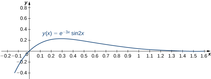
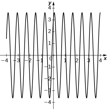
Solve the following initial-value problem and graph the solution:
We already solved this differential equation in [link]b. and found the general solution to be
Then
When
we have
and
Applying the initial conditions, we obtain
Therefore,
and the solution to the initial value problem is shown in the following graph.
Solve the following initial-value problem and graph the solution:
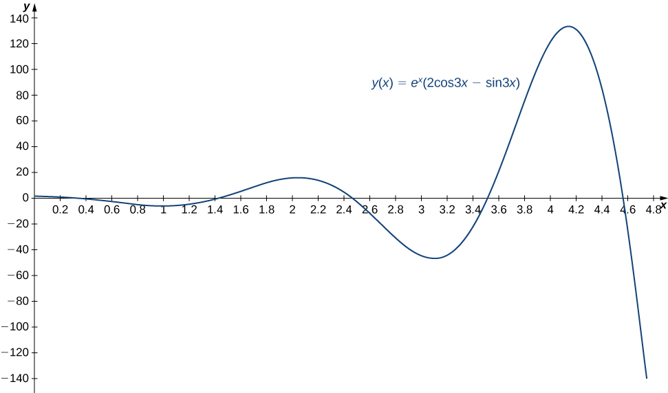
Hint
Use the initial conditions to determine values for
and
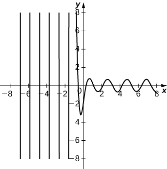
Initial-Value Problem Representing a Spring-Mass System
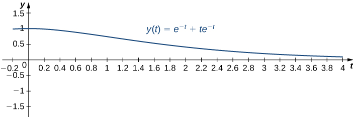
The following initial-value problem models the position of an object with mass attached to a spring. Spring-mass systems are examined in detail in Applications. The solution to the differential equation gives the position of the mass with respect to a neutral (equilibrium) position (in meters) at any given time. (Note that for spring-mass systems of this type, it is customary to define the downward direction as positive.)
Solve the initial-value problem and graph the solution. What is the position of the mass at time
sec? How fast is the mass moving at time
sec? In what direction?
In [link]c. we found the general solution to this differential equation to be
Then
When
we have
and
Applying the initial conditions, we obtain
Thus,
and the solution to the initial value problem is
This solution is represented in the following graph. At time
the mass is at position
m below equilibrium.
 To calculate the velocity at time
we need to find the derivative. We have
so
Then
At time
the mass is moving upward at 0.3679 m/sec.
Suppose the following initial-value problem models the position (in feet) of a mass in a spring-mass system at any given time. Solve the initial-value problem and graph the solution. What is the position of the mass at time
sec? How fast is it moving at time
sec? In what direction?
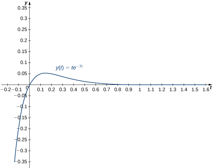
At time
The mass is 0.0367 ft below equilibrium. At time
The mass is moving downward at a speed of 0.1490 ft/sec.
Hint
Use the initial conditions to determine values for
and
Solving a Boundary-Value Problem
In [link]f. we solved the differential equation
and found the general solution to be
If possible, solve the boundary-value problem if the boundary conditions are the following:
-
-
-
We have
- Applying the first boundary condition given here, we get
So the solution is of the form
When we apply the second boundary condition, though, we get
for all values of
The boundary conditions are not sufficient to determine a value for
so this boundary-value problem has infinitely many solutions. Thus,
is a solution for any value of
- Applying the first boundary condition given here, we get
Applying the second boundary condition gives
so
In this case, we have a unique solution:
- Applying the first boundary condition given here, we get
However, applying the second boundary condition gives
so
We cannot have
so this boundary value problem has no solution.
Key Concepts
- Second-order differential equations can be classified as linear or nonlinear, homogeneous or nonhomogeneous.
- To find a general solution for a homogeneous second-order differential equation, we must find two linearly independent solutions. If
and
are linearly independent solutions to a second-order, linear, homogeneous differential equation, then the general solution is given by
- To solve homogeneous second-order differential equations with constant coefficients, find the roots of the characteristic equation. The form of the general solution varies depending on whether the characteristic equation has distinct, real roots; a single, repeated real root; or complex conjugate roots.
- Initial conditions or boundary conditions can then be used to find the specific solution to a differential equation that satisfies those conditions, except when there is no solution or infinitely many solutions.
Key Equations
- Linear second-order differential equation
- Second-order equation with constant coefficients
Classify each of the following equations as linear or nonlinear. If the equation is linear, determine whether it is homogeneous or nonhomogeneous.
For each of the following problems, verify that the given function is a solution to the differential equation. Use a graphing utility to graph the particular solutions for several values of c1 and c2. What do the solutions have in common?
[T]
[T]
[T]
[T]
Find the general solution to the linear differential equation.
Solve the initial-value problem.
Solve the boundary-value problem, if possible.
Find a differential equation with a general solution that is
Find a differential equation with a general solution that is
For each of the following differential equations:
- Solve the initial value problem.
- [T] Use a graphing utility to graph the particular solution.
a.
b.* * *
a.
b.* * *
(Principle of superposition) Prove that if
and
are solutions to a linear homogeneous differential equation,
then the function
where
and
are constants, is also a solution.
Prove that if a, b, and c are positive constants, then all solutions to the second-order linear differential equation
approach zero as
(Hint: Consider three cases: two distinct roots, repeated real roots, and complex conjugate roots.)
Glossary
- boundary conditions
- the conditions that give the state of a system at different times, such as the position of a spring-mass system at two different times
- boundary-value problem
- a differential equation with associated boundary conditions
- characteristic equation
- the equation
for the differential equation
- homogeneous linear equation
- a second-order differential equation that can be written in the form
but
for every value of
- nonhomogeneous linear equation
- a second-order differential equation that can be written in the form
but
for some value of
- linearly dependent
- a set of functions
for which there are constants
not all zero, such that
for all x in the interval of interest
- linearly independent
- a set of functions
for which there are no constants
such that
for all x in the interval of interest

This work is licensed under a Creative Commons Attribution 4.0 International License.
You can also download for free at http://cnx.org/contents/9a1df55a-b167-4736-b5ad-15d996704270@5.1
Attribution: