
Differential equations can be used to represent the size of a population as it varies over time. We saw this in an earlier chapter in the section on exponential growth and decay, which is the simplest model. A more realistic model includes other factors that affect the growth of the population. In this section, we study the logistic differential equation and see how it applies to the study of population dynamics in the context of biology.
To model population growth using a differential equation, we first need to introduce some variables and relevant terms. The variable
will represent time. The units of time can be hours, days, weeks, months, or even years. Any given problem must specify the units used in that particular problem. The variable
will represent population. Since the population varies over time, it is understood to be a function of time. Therefore we use the notation
for the population as a function of time. If
is a differentiable function, then the first derivative
represents the instantaneous rate of change of the population as a function of time.
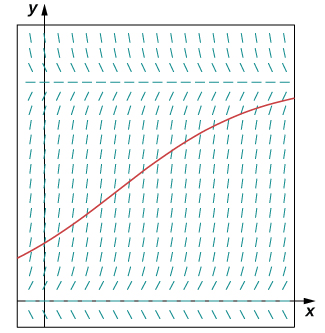
In Exponential Growth and Decay, we studied the exponential growth and decay of populations and radioactive substances. An example of an exponential growth function is
In this function,
represents the population at time
represents the initial population (population at time
and the constant
is called the growth rate. [link] shows a graph of
Here
and
We can verify that the function
satisfies the initial-value problem
This differential equation has an interesting interpretation. The left-hand side represents the rate at which the population increases (or decreases). The right-hand side is equal to a positive constant multiplied by the current population. Therefore the differential equation states that the rate at which the population increases is proportional to the population at that point in time. Furthermore, it states that the constant of proportionality never changes.
One problem with this function is its prediction that as time goes on, the population grows without bound. This is unrealistic in a real-world setting. Various factors limit the rate of growth of a particular population, including birth rate, death rate, food supply, predators, and so on. The growth constant
usually takes into consideration the birth and death rates but none of the other factors, and it can be interpreted as a net (birth minus death) percent growth rate per unit time. A natural question to ask is whether the population growth rate stays constant, or whether it changes over time. Biologists have found that in many biological systems, the population grows until a certain steady-state population is reached. This possibility is not taken into account with exponential growth. However, the concept of carrying capacity allows for the possibility that in a given area, only a certain number of a given organism or animal can thrive without running into resource issues.
The carrying capacity of an organism in a given environment is defined to be the maximum population of that organism that the environment can sustain indefinitely.
We use the variable
to denote the carrying capacity. The growth rate is represented by the variable
Using these variables, we can define the logistic differential equation.
Let
represent the carrying capacity for a particular organism in a given environment, and let
be a real number that represents the growth rate. The function
represents the population of this organism as a function of time
and the constant
represents the initial population (population of the organism at time
Then the logistic differential equation is
See this website for more information on the logistic equation.
The logistic equation was first published by Pierre Verhulst in
This differential equation can be coupled with the initial condition
to form an initial-value problem for
Suppose that the initial population is small relative to the carrying capacity. Then
is small, possibly close to zero. Thus, the quantity in parentheses on the right-hand side of [link] is close to
and the right-hand side of this equation is close to
If
then the population grows rapidly, resembling exponential growth.
However, as the population grows, the ratio
also grows, because
is constant. If the population remains below the carrying capacity, then
is less than
so
Therefore the right-hand side of [link] is still positive, but the quantity in parentheses gets smaller, and the growth rate decreases as a result. If
then the right-hand side is equal to zero, and the population does not change.
Now suppose that the population starts at a value higher than the carrying capacity. Then
and
Then the right-hand side of [link] is negative, and the population decreases. As long as
the population decreases. It never actually reaches
because
will get smaller and smaller, but the population approaches the carrying capacity as
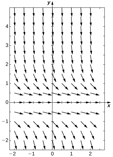
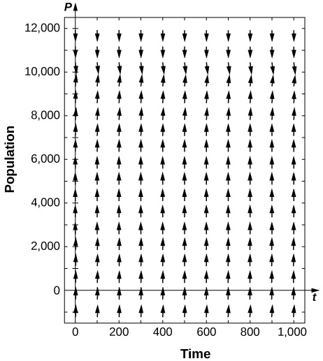
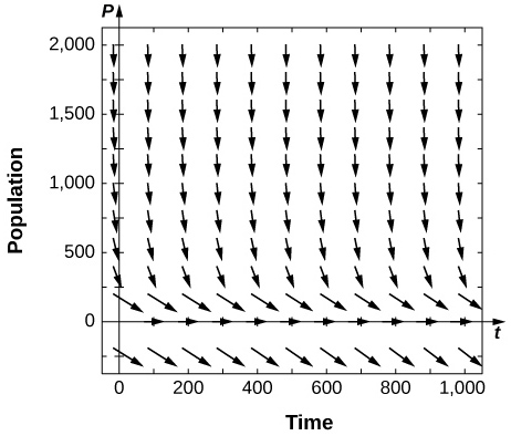
approaches infinity. This analysis can be represented visually by way of a phase line. A phase line describes the general behavior of a solution to an autonomous differential equation, depending on the initial condition. For the case of a carrying capacity in the logistic equation, the phase line is as shown in [link].
.")
This phase line shows that when
is less than zero or greater than
the population decreases over time. When
is between
and
the population increases over time.
") {:}
{:}
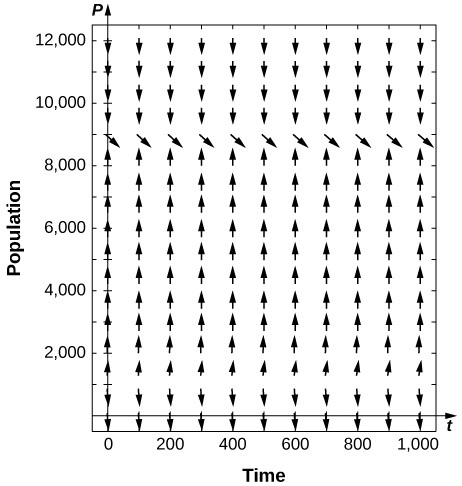
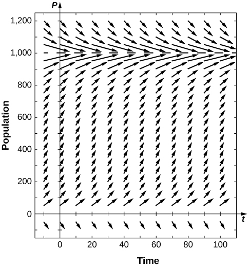
Let’s consider the population of white-tailed deer (Odocoileus virginianus) in the state of Kentucky. The Kentucky Department of Fish and Wildlife Resources (KDFWR) sets guidelines for hunting and fishing in the state. Before the hunting season of
it estimated a population of
deer. Johnson notes: “A deer population that has plenty to eat and is not hunted by humans or other predators will double every three years.” (George Johnson, “The Problem of Exploding Deer Populations Has No Attractive Solutions,” January
accessed April 9, 2015, http://www.txtwriter.com/onscience/Articles/deerpops.html.) This observation corresponds to a rate of increase
so the approximate growth rate is
per year. (This assumes that the population grows exponentially, which is reasonable––at least in the short term––with plentiful food supply and no predators.) The KDFWR also reports deer population densities for
counties in Kentucky, the average of which is approximately
deer per square mile. Suppose this is the deer density for the whole state
square miles). The carrying capacity
is
square miles times
deer per square mile, or
deer.
and
Substitute these values into [link] and form the initial-value problem.
years? Recall that the doubling time predicted by Johnson for the deer population was
years. How do these values compare?
deer. What does the logistic equation predict will happen to the population in this scenario?
Step 1: Setting the right-hand side equal to zero gives
and
This means that if the population starts at zero it will never change, and if it starts at the carrying capacity, it will never change.
Step 2: Rewrite the differential equation and multiply both sides by:
Divide both sides by
Step 3: Integrate both sides of the equation using partial fraction decomposition:
Step 4: Multiply both sides by
and use the quotient rule for logarithms:
Here
Next exponentiate both sides and eliminate the absolute value:
Here
but after eliminating the absolute value, it can be negative as well. Now solve for:
Step 5: To determine the value of
it is actually easier to go back a couple of steps to where
was defined. In particular, use the equation
The initial condition is
Replace
with
and
with zero:
Therefore
Dividing the numerator and denominator by
gives
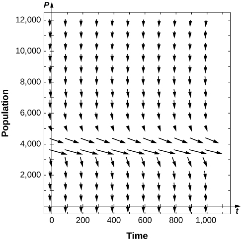
[link] is a graph of this equation.

years.
This is far short of twice the initial population of
Remember that the doubling time is based on the assumption that the growth rate never changes, but the logistic model takes this possibility into account.
deer, then the new initial-value problem would be
The general solution to the differential equation would remain the same.
To determine the value of the constant, return to the equation
Substituting the values
and
you get
Therefore
This equation is graphed in [link].

The logistic differential equation is an autonomous differential equation, so we can use separation of variables to find the general solution, as we just did in [link].
Step 1: Setting the right-hand side equal to zero leads to
and
as constant solutions. The first solution indicates that when there are no organisms present, the population will never grow. The second solution indicates that when the population starts at the carrying capacity, it will never change.
Step 2: Rewrite the differential equation in the form
Then multiply both sides by
and divide both sides by
This leads to
Multiply both sides of the equation by
and integrate:
The left-hand side of this equation can be integrated using partial fraction decomposition. We leave it to you to verify that
Then the equation becomes
Now exponentiate both sides of the equation to eliminate the natural logarithm:
We define
so that the equation becomes
To solve this equation for
first multiply both sides by
and collect the terms containing
on the left-hand side of the equation:
Next, factor
from the left-hand side and divide both sides by the other factor:
The last step is to determine the value of
The easiest way to do this is to substitute
and
in place of
in [link] and solve for
Finally, substitute the expression for
into [link]:
Now multiply the numerator and denominator of the right-hand side by
and simplify:
We state this result as a theorem.
Consider the logistic differential equation subject to an initial population of
with carrying capacity
and growth rate
The solution to the corresponding initial-value problem is given by
Now that we have the solution to the initial-value problem, we can choose values for
and
and study the solution curve. For example, in [link] we used the values
and an initial population of
deer. This leads to the solution
Dividing top and bottom by
gives
This is the same as the original solution. The graph of this solution is shown again in blue in [link], superimposed over the graph of the exponential growth model with initial population
and growth rate
(appearing in green). The red dashed line represents the carrying capacity, and is a horizontal asymptote for the solution to the logistic equation.

Working under the assumption that the population grows according to the logistic differential equation, this graph predicts that approximately
years earlier
the growth of the population was very close to exponential. The net growth rate at that time would have been around
per year. As time goes on, the two graphs separate. This happens because the population increases, and the logistic differential equation states that the growth rate decreases as the population increases. At the time the population was measured
it was close to carrying capacity, and the population was starting to level off.
The solution to the logistic differential equation has a point of inflection. To find this point, set the second derivative equal to zero:
Setting the numerator equal to zero,
As long as
the entire quantity before and including
is nonzero, so we can divide it out:
Solving for
Notice that if
then this quantity is undefined, and the graph does not have a point of inflection. In the logistic graph, the point of inflection can be seen as the point where the graph changes from concave up to concave down. This is where the “leveling off” starts to occur, because the net growth rate becomes slower as the population starts to approach the carrying capacity.
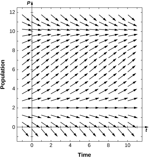
A population of rabbits in a meadow is observed to be
rabbits at time
After a month, the rabbit population is observed to have increased by
Using an initial population of
and a growth rate of
with a carrying capacity of
rabbits,
rabbits.
year.
After
months, the population will be
rabbits.
First determine the values of
and
Then create the initial-value problem, draw the direction field, and solve the problem.
An improvement to the logistic model includes a threshold population. The threshold population is defined to be the minimum population that is necessary for the species to survive. We use the variable
to represent the threshold population. A differential equation that incorporates both the threshold population
and carrying capacity
is
where
represents the growth rate, as before.
adults. (Catherine Clabby, “A Magic Number,” American Scientist 98(1): 24, doi:10.1511/2010.82.24. accessed April 9, 2015, http://www.americanscientist.org/issues/pub/a-magic-number). Therefore we use
as the threshold population in this project. Suppose that the environmental carrying capacity in Montana for elk is
Set up [link] using the carrying capacity of
and threshold population of
Assume an annual net growth rate of
along with several solutions for different initial populations. What are the constant solutions of the differential equation? What do these solutions correspond to in the original population model (i.e., in a biological context)?
(Hint: use the slope field to see what happens for various initial populations, i.e., look for the horizontal asymptotes of your solutions.)
Using an initial population of
elk, solve the initial-value problem and express the solution as an implicit function of
or solve the general initial-value problem, finding a solution in terms of
For the following problems, consider the logistic equation in the form
Draw the directional field and find the stability of the equilibria.
semi-stable
Solve the logistic equation for
and an initial condition of
Solve the logistic equation for
and an initial condition of
A population of deer inside a park has a carrying capacity of
and a growth rate of
If the initial population is
deer, what is the population of deer at any given time?
A population of frogs in a pond has a growth rate of
If the initial population is
frogs and the carrying capacity is
what is the population of frogs at any given time?
[T] Bacteria grow at a rate of
per hour in a petri dish. If there is initially one bacterium and a carrying capacity of
million cells, how long does it take to reach
cells?
hours
minutes
[T] Rabbits in a park have an initial population of
and grow at a rate of
per year. If the carrying capacity is
at what time does the population reach
rabbits?
[T] Two monkeys are placed on an island. After
years, there are
monkeys, and the estimated carrying capacity is
monkeys. When does the population of monkeys reach
monkeys?
years
months
[T] A butterfly sanctuary is built that can hold
butterflies, and
butterflies are initially moved in. If after
months there are now
butterflies, when does the population get to
butterflies?
The following problems consider the logistic equation with an added term for depletion, either through death or emigration.
[T] The population of trout in a pond is given by
where
trout are caught per year. Use your calculator or computer software to draw a directional field and draw a few sample solutions. What do you expect for the behavior?
In the preceding problem, what are the stabilities of the equilibria
[T] For the preceding problem, use software to generate a directional field for the value
What are the stabilities of the equilibria?
semi-stable
[T] For the preceding problems, use software to generate a directional field for the value
What are the stabilities of the equilibria?
[T] For the preceding problems, consider the case where a certain number of fish are added to the pond, or
What are the nonnegative equilibria and their stabilities?
stable
It is more likely that the amount of fishing is governed by the current number of fish present, so instead of a constant number of fish being caught, the rate is proportional to the current number of fish present, with proportionality constant
as
[T] For the previous fishing problem, draw a directional field assuming
Draw some solutions that exhibit this behavior. What are the equilibria and what are their stabilities?
[T] Use software or a calculator to draw directional fields for
What are the nonnegative equilibria and their stabilities?
is semi-stable
[T] Use software or a calculator to draw directional fields for
What are the equilibria and their stabilities?
Solve this equation, assuming a value of
and an initial condition of
fish.
Solve this equation, assuming a value of
and an initial condition of
fish.
The following problems add in a minimal threshold value for the species to survive,
which changes the differential equation to
Draw the directional field of the threshold logistic equation, assuming
When does the population survive? When does it go extinct?
For the preceding problem, solve the logistic threshold equation, assuming the initial condition
Bengal tigers in a conservation park have a carrying capacity of
and need a minimum of
to survive. If they grow in population at a rate of
per year, with an initial population of
tigers, solve for the number of tigers present.
A forest containing ring-tailed lemurs in Madagascar has the potential to support
individuals, and the lemur population grows at a rate of
per year. A minimum of
individuals is needed for the lemurs to survive. Given an initial population of
lemurs, solve for the population of lemurs.
The population of mountain lions in Northern Arizona has an estimated carrying capacity of
and grows at a rate of
per year and there must be
for the population to survive. With an initial population of
mountain lions, how many years will it take to get the mountain lions off the endangered species list (at least
years months
The following questions consider the Gompertz equation, a modification for logistic growth, which is often used for modeling cancer growth, specifically the number of tumor cells.
The Gompertz equation is given by
Draw the directional fields for this equation assuming all parameters are positive, and given that
Assume that for a population,
and
Draw the directional field associated with this differential equation and draw a few solutions. What is the behavior of the population?
Solve the Gompertz equation for generic
and
and
[T] The Gompertz equation has been used to model tumor growth in the human body. Starting from one tumor cell on day
and assuming
and a carrying capacity of
million cells, how long does it take to reach “detection” stage at
million cells?
days
[T] It is estimated that the world human population reached
billion people in
and
billion in
Assuming a carrying capacity of
billion humans, write and solve the differential equation for logistic growth, and determine what year the population reached
billion.
[T] It is estimated that the world human population reached
billion people in
and
billion in
Assuming a carrying capacity of
billion humans, write and solve the differential equation for Gompertz growth, and determine what year the population reached
billion. Was logistic growth or Gompertz growth more accurate, considering world population reached
billion on October
September
Show that the population grows fastest when it reaches half the carrying capacity for the logistic equation
When does population increase the fastest in the threshold logistic equation
When does population increase the fastest for the Gompertz equation
Below is a table of the populations of whooping cranes in the wild from
The population rebounded from near extinction after conservation efforts began. The following problems consider applying population models to fit the data. Assume a carrying capacity of
cranes. Fit the data assuming years since
(so your initial population at time
would be
cranes).
| Year (years since conservation began) | Whooping Crane Population |
|---|---|
Find the equation and parameter
that best fit the data for the logistic equation.
Find the equation and parameters
and
that best fit the data for the threshold logistic equation.
Find the equation and parameter
that best fit the data for the Gompertz equation.
Graph all three solutions and the data on the same graph. Which model appears to be most accurate?
Using the three equations found in the previous problems, estimate the population in
(year
after conservation). The real population measured at that time was
Which model is most accurate?
Logistic:
Threshold:
Gompertz:
in the exponential growth function
and growth rate
into a population model

You can also download for free at http://cnx.org/contents/9a1df55a-b167-4736-b5ad-15d996704270@5.1
Attribution: