=−0.4(T−72). Two solutions are plotted: one with initial temperature less than 72°F and the other with initial temperature greater than 72°F.")
For the rest of this chapter we will focus on various methods for solving differential equations and analyzing the behavior of the solutions. In some cases it is possible to predict properties of a solution to a differential equation without knowing the actual solution. We will also study numerical methods for solving differential equations, which can be programmed by using various computer languages or even by using a spreadsheet program, such as Microsoft Excel.
Direction fields (also called slope fields) are useful for investigating first-order differential equations. In particular, we consider a first-order differential equation of the form
An applied example of this type of differential equation appears in Newton’s law of cooling, which we will solve explicitly later in this chapter. First, though, let us create a direction field for the differential equation
Here
represents the temperature (in degrees Fahrenheit) of an object at time
and the ambient temperature is
[link] shows the direction field for this equation.
The idea behind a direction field is the fact that the derivative of a function evaluated at a given point is the slope of the tangent line to the graph of that function at the same point. Other examples of differential equations for which we can create a direction field include
To create a direction field, we start with the first equation:
We let
be any ordered pair, and we substitute these numbers into the right-hand side of the differential equation. For example, if we choose
substituting into the right-hand side of the differential equation yields
This tells us that if a solution to the differential equation
passes through the point
then the slope of the solution at that point must equal
To start creating the direction field, we put a short line segment at the point
having slope
We can do this for any point in the domain of the function
which consists of all ordered pairs
in
Therefore any point in the Cartesian plane has a slope associated with it, assuming that a solution to the differential equation passes through that point. The direction field for the differential equation
is shown in [link].

We can generate a direction field of this type for any differential equation of the form
A direction field (slope field) is a mathematical object used to graphically represent solutions to a first-order differential equation. At each point in a direction field, a line segment appears whose slope is equal to the slope of a solution to the differential equation passing through that point.
We can use a direction field to predict the behavior of solutions to a differential equation without knowing the actual solution. For example, the direction field in [link] serves as a guide to the behavior of solutions to the differential equation
To use a direction field, we start by choosing any point in the field. The line segment at that point serves as a signpost telling us what direction to go from there. For example, if a solution to the differential equation passes through the point
then the slope of the solution passing through that point is given by
Now let
increase slightly, say to
Using the method of linear approximations gives a formula for the approximate value of
for
In particular,
Substituting
into
gives an approximate
value of
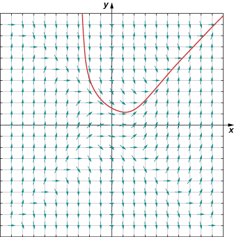
At this point the slope of the solution changes (again according to the differential equation). We can keep progressing, recalculating the slope of the solution as we take small steps to the right, and watching the behavior of the solution. [link] shows a graph of the solution passing through the point
.")
The curve is the graph of the solution to the initial-value problem
This curve is called a solution curve passing through the point
The exact solution to this initial-value problem is
and the graph of this solution is identical to the curve in [link].
Create a direction field for the differential equation
and sketch a solution curve passing through the point
Use
and
values ranging from
to
For each coordinate pair, calculate
using the right-hand side of the differential equation.
Go to this Java applet and this website to see more about slope fields.
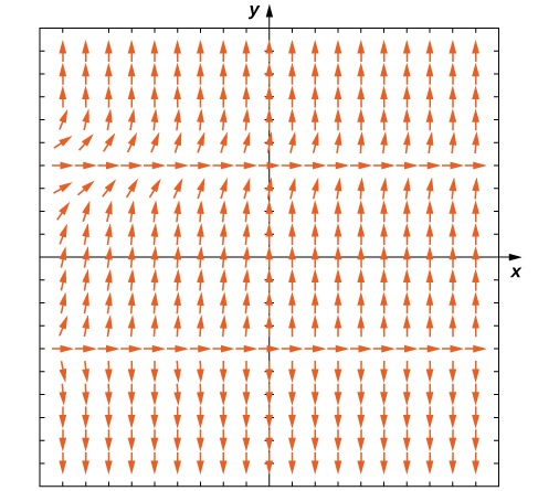
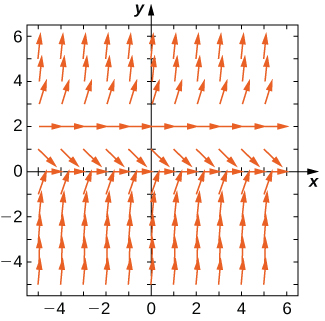
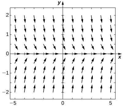
Now consider the direction field for the differential equation
shown in [link]. This direction field has several interesting properties. First of all, at
and
horizontal dashes appear all the way across the graph. This means that if
then
Substituting this expression into the right-hand side of the differential equation gives
Therefore
is a solution to the differential equation. Similarly,
is a solution to the differential equation. These are the only constant-valued solutions to the differential equation, as we can see from the following argument. Suppose
is a constant solution to the differential equation. Then
Substituting this expression into the differential equation yields
This equation must be true for all values of
so the second factor must equal zero. This result yields the equation
The solutions to this equation are
and
which are the constant solutions already mentioned. These are called the equilibrium solutions to the differential equation.
(y2−4) showing two solutions. These solutions are very close together, but one is barely above the equilibrium solution x=−2 and the other is barely below the same equilibrium solution.")
Consider the differential equation
An equilibrium solution is any solution to the differential equation of the form
where
is a constant.
To determine the equilibrium solutions to the differential equation
set the right-hand side equal to zero. An equilibrium solution of the differential equation is any function of the form
such that
for all values of
in the domain of
An important characteristic of equilibrium solutions concerns whether or not they approach the line
as an asymptote for large values of
Consider the differential equation
and assume that all solutions to this differential equation are defined for
Let
be an equilibrium solution to the differential equation.
is an asymptotically stable solution to the differential equation if there exists
such that for any value
the solution to the initial-value problem
approaches
as
approaches infinity.
is an asymptotically unstable solution to the differential equation if there exists
such that for any value
the solution to the initial-value problem
never approaches
as
approaches infinity.
is an asymptotically semi-stable solution to the differential equation if it is neither asymptotically stable nor asymptotically unstable.
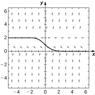
Now we return to the differential equation
with the initial condition
The direction field for this initial-value problem, along with the corresponding solution, is shown in [link].
(y2−4),y(0)=0.5.")
The values of the solution to this initial-value problem stay between
and
which are the equilibrium solutions to the differential equation. Furthermore, as
approaches infinity,
approaches
The behavior of solutions is similar if the initial value is higher than
for example,
In this case, the solutions decrease and approach
as
approaches infinity. Therefore
is an asymptotically stable solution to the differential equation.
What happens when the initial value is below
This scenario is illustrated in [link], with the initial value
(y2−4),y(0)=−3.")
The solution decreases rapidly toward negative infinity as
approaches infinity. Furthermore, if the initial value is slightly higher than
then the solution approaches
which is the other equilibrium solution. Therefore in neither case does the solution approach
so
is called an asymptotically unstable, or unstable, equilibrium solution.
Create a direction field for the differential equation
and identify any equilibrium solutions. Classify each of the equilibrium solutions as stable, unstable, or semi-stable.
The direction field is shown in [link].
2(y2+y−2).")
The equilibrium solutions are
and
To classify each of the solutions, look at an arrow directly above or below each of these values. For example, at
the arrows directly below this solution point up, and the arrows directly above the solution point down. Therefore all initial conditions close to
approach
and the solution is stable. For the solution
all initial conditions above and below
are repelled (pushed away) from
so this solution is unstable. The solution
is semi-stable, because for initial conditions slightly greater than
the solution approaches infinity, and for initial conditions slightly less than
the solution approaches
It is possible to find the equilibrium solutions to the differential equation by setting the right-hand side equal to zero and solving for
This approach gives the same equilibrium solutions as those we saw in the direction field.
Create a direction field for the differential equation
and identify any equilibrium solutions. Classify each of the equilibrium solutions as stable, unstable, or semi-stable.
The equilibrium solutions are
and
For this equation,
is an unstable equilibrium solution, and
is a semi-stable equilibrium solution.
First create the direction field and look for horizontal dashes that go all the way across. Then examine the slope lines directly above and below the equilibrium solutions.
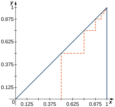
Consider the initial-value problem
Integrating both sides of the differential equation gives
and solving for
yields the particular solution
The solution for this initial-value problem appears as the parabola in [link].
![A graph over the range [-1,4] for x and y. The given upward opening parabola is drawn with vertex at (1.5, 0.75). Individual points are plotted at (0, 3), (0.5, 1.5), (1, 0.5), (1.5, 0), (2, 0), (2.5, 0.5), and (3, 1.5) with line segments connecting them.](../resources/CNX_Calc_Figure_08_02_010.jpg "Euler’s Method for the initial-value problem y′=2x−3,y(0)=3.")
The red graph consists of line segments that approximate the solution to the initial-value problem. The graph starts at the same initial value of
Then the slope of the solution at any point is determined by the right-hand side of the differential equation, and the length of the line segment is determined by increasing the
value by
each time (the step size). This approach is the basis of Euler’s Method.
Before we state Euler’s Method as a theorem, let’s consider another initial-value problem:
The idea behind direction fields can also be applied to this problem to study the behavior of its solution. For example, at the point
the slope of the solution is given by
so the slope of the tangent line to the solution at that point is also equal to
Now we define
and
Since the slope of the solution at this point is equal to
we can use the method of linear approximation to approximate
near
Here
and
so the linear approximation becomes
Now we choose a step size. The step size is a small value, typically
or less, that serves as an increment for
it is represented by the variable
In our example, let
Incrementing
by
gives our next
value:
We can substitute
into the linear approximation to calculate
Therefore the approximate
value for the solution when
is
We can then repeat the process, using
and
to calculate
and
The new slope is given by
First,
Using linear approximation gives
Finally, we substitute
into the linear approximation to calculate
Therefore the approximate value of the solution to the differential equation is
when
What we have just shown is the idea behind Euler’s Method. Repeating these steps gives a list of values for the solution. These values are shown in [link], rounded off to four decimal places.
Consider the initial-value problem
To approximate a solution to this problem using Euler’s method, define
Here
represents the step size and
is an integer, starting with
The number of steps taken is counted by the variable
Typically
is a small value, say
or
The smaller the value of
the more calculations are needed. The higher the value of
the fewer calculations are needed. However, the tradeoff results in a lower degree of accuracy for larger step size, as illustrated in [link].
=3 with (a) a step size of h=0.5; and (b) a step size of h=0.25.")
Consider the initial-value problem
Use Euler’s method with a step size of
to generate a table of values for the solution for values of
between
and
We are given
and
Furthermore, the initial condition
gives
and
Using [link] with
we can generate [link].
With ten calculations, we are able to approximate the values of the solution to the initial-value problem for values of
between
and
For more information on Euler's method use this applet.
Consider the initial-value problem
Using a step size of
generate a table with approximate values for the solution to the initial-value problem for values of
between
and
| {: valign=”top”} | ———- |
| {: valign=”top”} |
| {: valign=”top”} |
| {: valign=”top”} |
| {: valign=”top”} |
| {: valign=”top”} |
| {: valign=”top”} |
| {: valign=”top”} |
| {: valign=”top”} |
| {: valign=”top”} |
| {: valign=”top”} |
| {: valign=”top”}{: .unnumbered summary=”A table with three columns and eleven rows. The first column has the header n and the values 0 through 10. The second column has the header x_n and the values 1 through 2, increasing by 0.1. The third column has the header y_n = y_(n - 1) + hf(x_(n - 1), y_(n - 1)) and the values -2, -1.5, -1.1419, -0.8387, -0.5487, -0.2442, 0.0993, 0.5099, 1.0272, 1.7159, and 2.6962.” data-label=””}
Start by identifying the value of
then figure out what
is. Then use the formula for Euler’s Method to calculate
and so on.
Visit this website for a practical application of the material in this section.
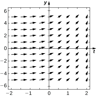
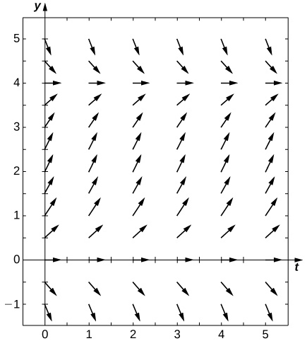
For the following problems, use the direction field below from the differential equation
Sketch the graph of the solution for the given initial conditions.* * *
Are there any equilibria? What are their stabilities?
is a stable equilibrium
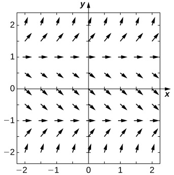
For the following problems, use the direction field below from the differential equation
Sketch the graph of the solution for the given initial conditions.* * *
Are there any equilibria? What are their stabilities?
is a stable equilibrium and
is unstable
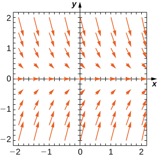
Draw the direction field for the following differential equations, then solve the differential equation. Draw your solution on top of the direction field. Does your solution follow along the arrows on your direction field?
![A direction field over [-2, 2] in the x and y axes. The arrows point slightly down and to the right over [-2, 0] and gradually become vertical over [0, 2].](../resources/CNX_Calc_Figure_08_02_212.jpg)
Draw the directional field for the following differential equations. What can you say about the behavior of the solution? Are there equilibria? What stability do these equilibria have?
![A direction field with arrows pointing down and to the right for nearly all points in [-2, 2] on the x and y axes. Close to the origin, the arrows become more horizontal, point to the upper right, become more horizontal, and then point down to the right again.](../resources/CNX_Calc_Figure_08_02_216.jpg)
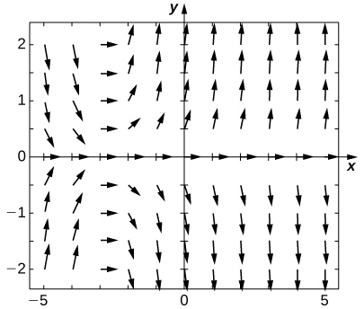
Match the direction field with the given differential equations. Explain your selections.* * *
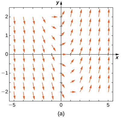
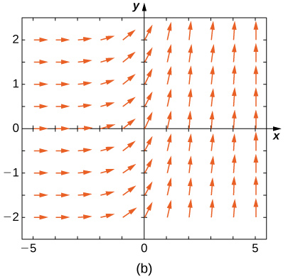
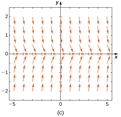
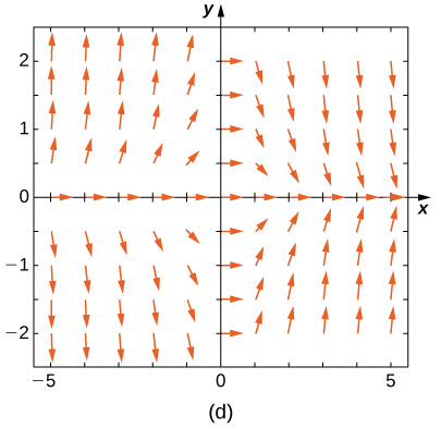
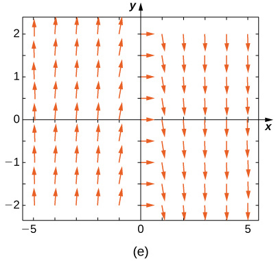
E
A
Match the direction field with the given differential equations. Explain your selections.* * *
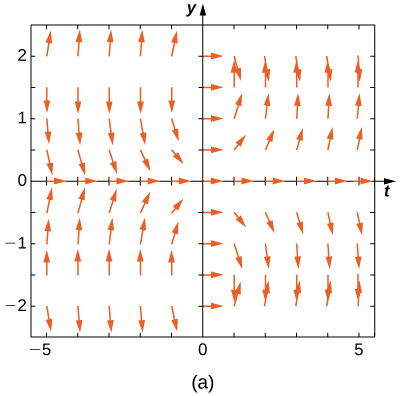
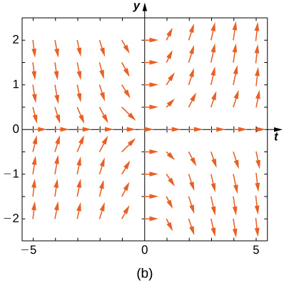
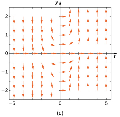
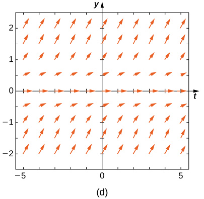
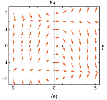
B
A
C
Estimate the following solutions using Euler’s method with
steps over the interval
If you are able to solve the initial-value problem exactly, compare your solution with the exact solution. If you are unable to solve the initial-value problem, the exact solution will be provided for you to compare with Euler’s method. How accurate is Euler’s method?
exact:
Exact solution is
Exact solution is
exact:
[T]
Exact solution is
exact:
Exact solution is
Exact solution is
exact:
Exact solution is
Exact solution is
exact:
Differential equations can be used to model disease epidemics. In the next set of problems, we examine the change of size of two sub-populations of people living in a city: individuals who are infected and individuals who are susceptible to infection.
represents the size of the susceptible population, and
represents the size of the infected population. We assume that if a susceptible person interacts with an infected person, there is a probability
that the susceptible person will become infected. Each infected person recovers from the infection at a rate
and becomes susceptible again. We consider the case of influenza, where we assume that no one dies from the disease, so we assume that the total population size of the two sub-populations is a constant number,
The differential equations that model these population sizes are
Here
represents the contact rate and
is the recovery rate.
Show that, by our assumption that the total population size is constant
you can reduce the system to a single differential equation in
Assuming the parameters are
and
draw the resulting directional field.
[T] Use computational software or a calculator to compute the solution to the initial-value problem
using Euler’s Method with the given step size
Find the solution at
For a hint, here is “pseudo-code” for how to write a computer program to perform Euler’s Method for
Create function
Define parameters
step size
and total number of steps,
Write a for loop:
for
Solve the initial-value problem for the exact solution.
Draw the directional field
[T]
[T]
[T]
[T] Evaluate the exact solution at
Make a table of errors for the relative error between the Euler’s method solution and the exact solution. How much does the error change? Can you explain?
| Step Size | Error |
| {: valign=”top”} | ———- |
| {: valign=”top”} |
| {: valign=”top”} |
| {: valign=”top”} |
| {: valign=”top”}{: .unnumbered summary=”A table with two columns and five rows. The first column contains the label “Step Size” and the values h = 1, h=10, h=100, and h=1000. The second column contains the label “Error” and the values 0.3935, 0.06163, 0.006612, and 0.0006661.” data-label=””}
Consider the initial-value problem
Show that
solves this initial-value problem.
Draw the directional field of this differential equation.
[T] By hand or by calculator or computer, approximate the solution using Euler’s Method at
using
[T] By calculator or computer, approximate the solution using Euler’s Method at
using
[T] Plot exact answer and each Euler approximation (for
and
at each
on the directional field. What do you notice?
if it is neither asymptotically stable nor asymptotically unstable
if there exists
such that for any value
the solution to the initial-value problem
approaches
as
approaches infinity
if there exists
such that for any value
the solution to the initial-value problem
never approaches
as
approaches infinity
where
is a constant
that is added to the
value at each step in Euler’s Method

You can also download for free at http://cnx.org/contents/9a1df55a-b167-4736-b5ad-15d996704270@5.1
Attribution: