
Many real-world phenomena can be modeled mathematically by using differential equations. Population growth, radioactive decay, predator-prey models, and spring-mass systems are four examples of such phenomena. In this chapter we study some of these applications.
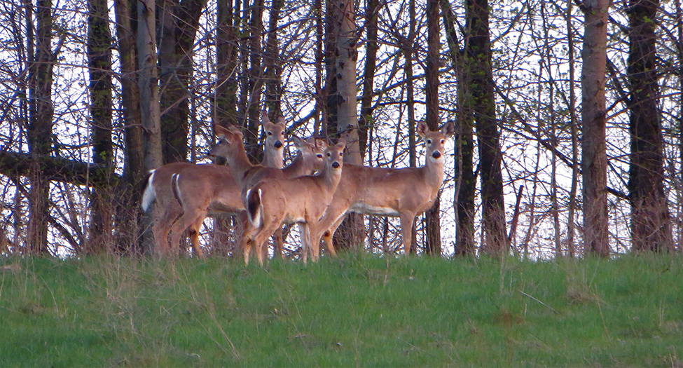
Suppose we wish to study a population of deer over time and determine the total number of animals in a given area. We can first observe the population over a period of time, estimate the total number of deer, and then use various assumptions to derive a mathematical model for different scenarios. Some factors that are often considered are environmental impact, threshold population values, and predators. In this chapter we see how differential equations can be used to predict populations over time (see [link]).
Another goal of this chapter is to develop solution techniques for different types of differential equations. As the equations become more complicated, the solution techniques also become more complicated, and in fact an entire course could be dedicated to the study of these equations. In this chapter we study several types of differential equations and their corresponding methods of solution.

You can also download for free at http://cnx.org/contents/9a1df55a-b167-4736-b5ad-15d996704270@5.1
Attribution: